Welcome back to our mini-series on quantum probability! Last time, we motivated the series by pondering over a thought from classical probability theory, namely that marginal probability doesn't have memory. That is, the process of summing over of a variable in a joint probability distribution causes information about that variable to be lost. But as we saw then, there is a quantum version of marginal probability that behaves much like "marginal probability with memory." It remembers what's destroyed when computing marginals in the usual way. In today's post, I'll unveil the details. Along the way, we'll take an introductory look at the mathematics of quantum probability theory.

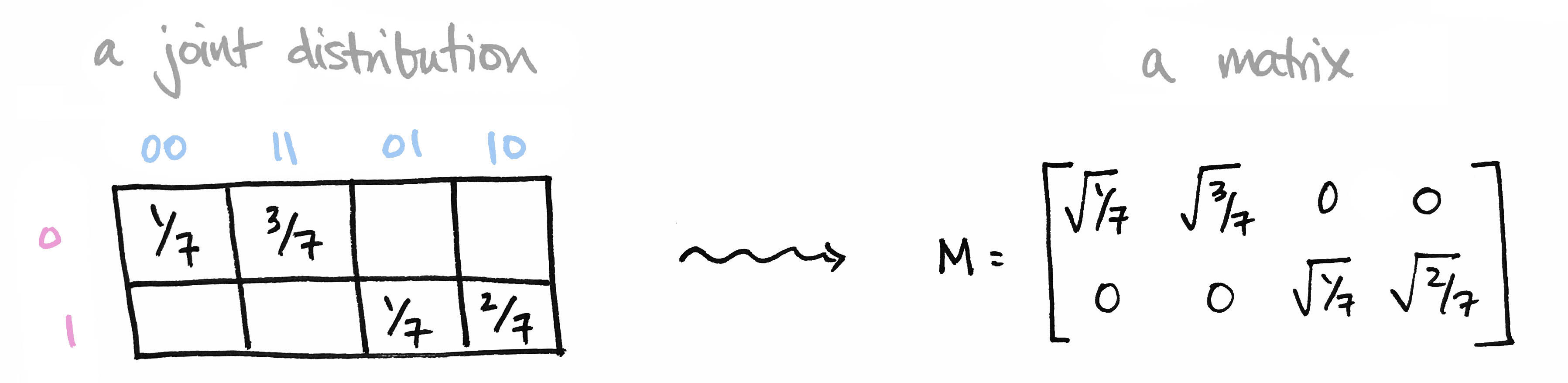
Let's begin with a brief recap of the ideas covered in Part 1: We began with a joint probability distribution on a product of finite sets $p\colon X\times Y\to [0,1]$ and realized it as a matrix $M$ by setting $M_{ij} = \sqrt{p(x_i),p(y_j)}$. We called elements of our set $X=\{0,1\}$ prefixes and the elements of our set $Y=\{00,11,01,10\}$ suffixes so that $X\times Y$ is the set of all bitstrings of length 3.

We then observed that the matrix $M^\top M$ contains the marginal probability distribution of $Y$ along its diagonal. Moreover its eigenvectors define conditional probability distributions on $Y$. Likewise, $MM^\top$ contains marginals on $X$ along its diagonal, and its eigenvectors define conditional probability distributions on $X$.

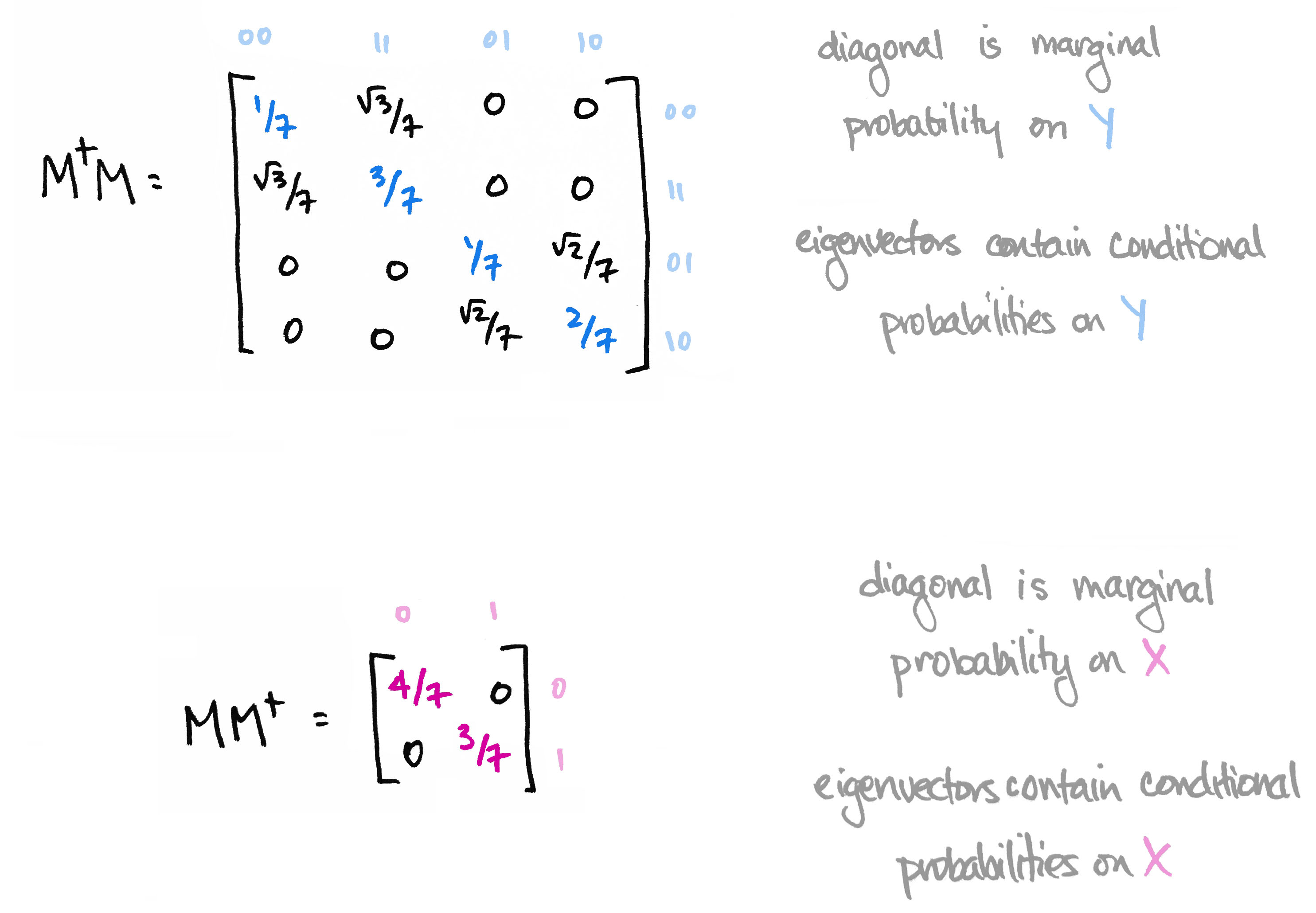
The information in the eigenvectors of $M^\top M$ and $MM^\top$ is precisely the information that's  destroyed when computing marginal probability in the usual way. The big reveal last time was that the matrices $M^\top M$ and $MM^\top$ are the quantum versions of marginal probability distributions.

As we'll see today, the quantum version of a probability distribution is something called a density operator. The quantum version of marginalizing corresponds to "reducing" that operator to a subsystem. This reduction is a construction in linear algebra called the partial trace. I'll start off by explaining the partial trace. Then I'll introduce the basics of quantum probability theory. At the end, we'll tie it all back to our bitstring example.

In this article and the next, I'd like to share some ideas from the world of quantum probability.* The word "quantum" is pretty loaded, but don't let that scare you. We'll take a first—not second or third—look at the subject, and the only prerequisites will be linear algebra and basic probability. In fact, I like to think of quantum probability as another name for "linear algebra + probability," so this mini-series will explore the mathematics, rather than the physics, of the subject.**

In today's post, we'll motivate the discussion by saying a few words about (classical) probability. In particular, let's spend a few moments thinking about the following: ‍

What do I mean? We'll start with some basic definitions. Then I'll share an example that illustrates this idea.

A probability distribution (or simply, distribution) on a finite set $X$ is a function $p \colon X\to [0,1]$ satisfying $\sum_x p(x) = 1$. I'll use the term joint probability distribution to refer to a distribution on a Cartesian product of finite sets, i.e. a function $p\colon X\times Y\to [0,1]$ satisfying $\sum_{(x,y)}p(x,y)=1$. Every joint distribution defines a marginal probability distribution on one of the sets by summing probabilities over the other set. For instance, the marginal distribution $p_X\colon X\to [0,1]$ on $X$ is defined by $p_X(x)=\sum_yp(x,y)$, in which the variable $y$ is summed, or "integrated," out. It's this very process of summing or integrating out that causes information to be lost. In other words, marginalizing loses information. It doesn't remember what was summed away!

I'll illustrate this with a simple example. To do so, I need to give you some finite sets $X$ and $Y$ and a probability distribution on them.