A First Look at Quantum Probability, Part 2

Welcome back to our mini-series on quantum probability! Last time, we motivated the series by pondering over a thought from classical probability theory, namely that marginal probability doesn't have memory. That is, the process of summing over of a variable in a joint probability distribution causes information about that variable to be lost. But as we saw then, there is a quantum version of marginal probability that behaves much like "marginal probability with memory." It remembers what's destroyed when computing marginals in the usual way. In today's post, I'll unveil the details. Along the way, we'll take an introductory look at the mathematics of quantum probability theory.

Let's begin with a brief recap of the ideas covered in Part 1: We began with a joint probability distribution on a product of finite sets $p\colon X\times Y\to [0,1]$ and realized it as a matrix $M$ by setting $M_{ij} = \sqrt{p(x_i,y_j)}$. We called elements of our set $X=\{0,1\}$ prefixes and the elements of our set $Y=\{00,11,01,10\}$ suffixes so that $X\times Y$ is the set of all bitstrings of length 3.

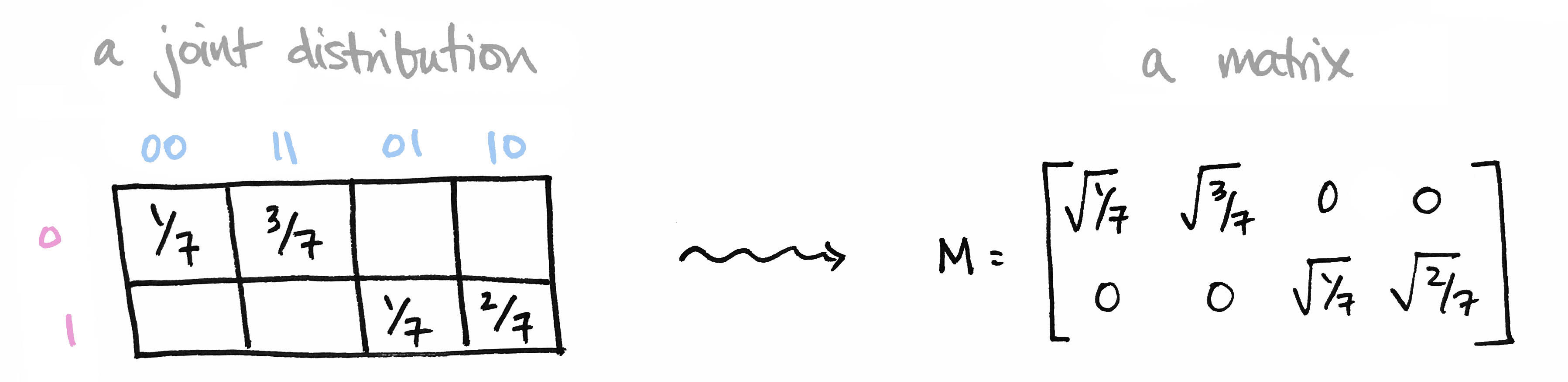
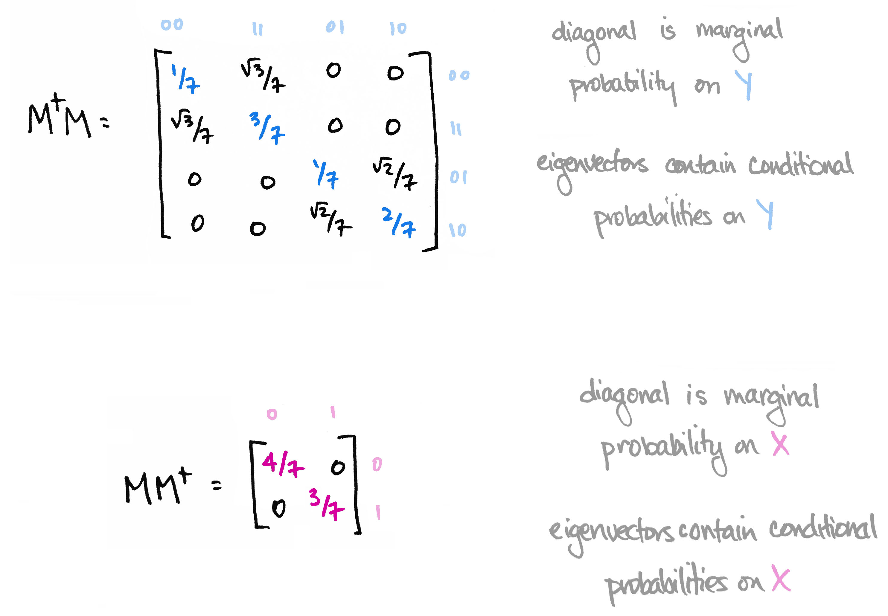
We then observed that the matrix $M^\top M$ contains the marginal probability distribution of $Y$ along its diagonal. Moreover its eigenvectors define conditional probability distributions on $Y$. Likewise, $MM^\top$ contains marginals on $X$ along its diagonal, and its eigenvectors define conditional probability distributions on $X$.

The information in the eigenvectors of $M^\top M$ and $MM^\top$ is precisely the information that's  destroyed when computing marginal probability in the usual way. The big reveal last time was that the matrices $M^\top M$ and $MM^\top$ are the quantum versions of marginal probability distributions.

As we'll see today, the quantum version of a probability distribution is something called a density operator. The quantum version of marginalizing corresponds to "reducing" that operator to a subsystem. This reduction is a construction in linear algebra called the partial trace. I'll start off by explaining the partial trace. Then I'll introduce the basics of quantum probability theory. At the end, we'll tie it all back to our bitstring example.

Introducing: The Partial Trace

I'll begin by citing a fact from linear algebra. It's a fact about the tensor product of vector spaces $V\otimes W$. (New to tensor products? I've written a friendly introduction here.) Here it is:

‍Fact: There are no natural linear maps from the tensor product down to each factor.

‍You can try to project $v\otimes w\in V\otimes W$ to $v\in V$, for example, but that function isn't linear. Happily, this problem is corrected once we pass to endomorphisms of the spaces. (An "endomorphism" on a space $V$ is another name for a linear map from $V$ to itself.) That is, there are natural linear maps out of endomorphisms on a tensor product down to endomorphisms of each factor. These maps are called partial traces.

If $f$, for instance, is an operator on $V$ and if $g$ is an operator on $W$ then the partial trace $tr_V$ takes the operator $f\otimes g$ on $V\otimes W$ and produces $tr_V(f\otimes g) = g\cdot tr(f)$, which is an operator on $W$ alone. It's just $g$ multiplied by the trace of $f$! You could say we've "traced out" the system $V$. We could also "trace out $W$" to get an operator on $V$ alone: $tr_W(f\otimes g) = f\cdot tr(g)$.

So unlike the trace, which takes a linear operator and produces a number, the partial trace takes an operator and produces another operator—one that operates on a smaller space. The partial trace also has a basis-dependent definition, which can be understood visually with tensor diagram notation. (Check out this post for an introduction to tensor diagrams.)

The partial trace reminds me of people-watching at the park on a busy day. Lots of folks might be bustling around, but you can hone in on a few of them and learn something as they interact with their surroundings. You can likewise learn something about an operator by observing how a smaller piece of it interacts with its environment. The partial trace provides a way to do this. This comes in handy if you have an operator on a huge tensor product $V_1\otimes V_2\otimes\cdots\otimes V_N$, a big conglomeration that might be too much to work with. The linear algebra allows us to hone in on a smaller chunk of the system—say, just the first couple of factors, $V_1\otimes V_2$—and learn something about it, given that it's a part of and interacts with a larger system.

How, then, does the partial trace relate to our bitstring example? As we'll see below, the two matrices $M^\top M$ and $MM^\top$—whose diagonals contain marginal probabilities and whose eigenvectors contain additional information—are operators obtained by partial traces. In this way, the partial trace is the quantum version of marginalizing.

To better understand this, we first need some basic definitions from quantum probability theory. Indeed, it will be good to understand the quantum version of a probability distribution before exploring the quantum version of a marginal probability distribution.

The basics of quantum probability

Here's a picture of a quantum particle:

The state of this particle is defined to be a linear operator on a Hilbert space. (A Hilbert space is a vector space with an inner product; you can think of $\mathbb{C}^n$ with the dot product if you like. We'll only consider finite-dimensional spaces.) But not just any linear operator. It must satisfy three properties, which amount to the quantum version of probability distribution. Such operators are given a special name: density operators.

The quantum version of a probability distribution is a density operator, i.e. a Hermitian, positive semidefinite operator with trace equal to one. In physics lingo, this is called a quantum state.

Let me say a few words about this.

First, here's why "Hermitian + positive semidefinite + trace one" amounts to the quantum analogue of a probability distribution:

1. Hermitian: An operator is Hermitian if it's equal to its conjugate transpose. The eigenvalues of a Hermitian operator are always real. This is analogous to the fact that probabilities are real—not complex—numbers.
2. Positive semidefinite: An operator $f\colon V\to V$ is positive semidefinite if $\langle v,fv\rangle \geq 0$ for all $v\in V$, which is to say that $f$ doesn't cause any vector $v$ to point "opposite" of the direction it was originally pointing in, before $f$'s transformation. The eigenvalues of a positive semidefinite operator are always non-negative. This is analogous to the fact that probabilities are non-negative.
3. Unit trace: The trace of an operator is the sum of the diagonal entries of a matrix representing it. The trace is also equal to the sum of the eigenvalues of the operator. We ask for the trace of a density operator to be 1. This is analogous to the fact that the values in a probability distribution add up to 1.

The connection between classical and quantum probability can be made even sharper: every classical distribution defines a quantum state, and every quantum state defines a classical distribution. This provides a passage between them: classical $\leftrightsquigarrow$ quantum. It's worth exploring, so let's take a brief interlude.

Interlude: Classical $\leftrightsquigarrow$ Quantum

Every classical probability distribution $p\colon X\to [0,1]$ defines a density operator $\rho_p$ on $\mathbb{C}^X$. In fact, it does so in more than one way. Here's one way: simply write down a matrix with the probabilities along its diagonal.

The eigenvalues of this matrix are its diagonal entries, and indeed those entries are nonnegative, and add up to 1. This matrix is thus Hermitian, positive semidefinite, and has unit trace. So these three properties capture classical probability nicely.

But there's another way to turn a classical probability distribution into a density operator, and I think it's much more interesting: Think of your distribution $(p(x_1),\ldots,p(x_n))$ as a point in $n$-dimensional space. Now take the square root of each probability to get a new point $(\sqrt{p(x_1)},\ldots, \sqrt{p(x_n)})$. This point defines a line passing through the origin. Orthogonal projection onto that line is a density operator.

This setup is worth understanding well, so let me describe it more carefully.

Every probability distribution defines a quantum state.

The passage from classical probability theory to quantum probability theory is really just a passage from sets to vector spaces. To see this, let $X$ be a finite set and let $p\colon X\to[0,1]$ be a probability distribution on $X$. Let $\mathbb{C}^X$ denote the free vector space on $X$. If we choose an ordering $X=\{x_1,\ldots,x_n\}$ then we can think of each element $x_i$ as an $n\times 1$ basis vector $\mathbf{x}_i$ that has a 1 in the $i$th entry and zeros elsewhere. This space has a natural inner product: define $\langle \mathbf{x}_i,\mathbf{x}_j\rangle$ to be one if $i=j$ and zero otherwise. In this way $X$ forms an orthonormal basis and $\mathbb{C}^X$ is a Hilbert space. The probability distribution $p$ then defines a quantum state $\rho_p$ on $\mathbb{C}^X$ in the two ways described above:

• First way: a diagonal operator. Let $\text{Proj}_{\mathbf{x}_i}$ denote orthogonal projection onto the vector $\mathbf{x}_i$ and define $\rho_p=\sum_i p(x_i)\text{Proj}_{\mathbf{x}_i}$. As a matrix, this has the probabilities along its diagonal and zeros everywhere else.
• Second way: orthogonal projection. Let $\psi=\sum_i\sqrt{p(x_i)}\mathbf{x}_i\in \mathbb{C}^X$ and define $\rho_p= \psi\otimes \psi^*$ where $\psi^*$ denotes the dual of $\psi$. As a matrix, this is $\psi \psi^\top$.

Both densities satisfy the Born rule equation $p(x) = \langle \mathbf{x} , \rho\mathbf{x}\rangle$. You could define other densities from $p$ which will also satisfy this equation, but think of these as two extremes: the diagonal operator has maximal rank, orthogonal projection has minimal rank, and others will lie somewhere in between.

Both of these constructions works for joint probability distributions, too. If $p$ is a probability distribution on a Cartesian product $X\times Y$ then the induced density $\rho_p$ will be an operator on $\mathbb{C}^{X\times Y}$ which is isomorphic to the tensor product $\mathbb{C}^X\otimes\mathbb{C}^Y$.

In particular, the joint distribution on our set of bitstrings in Part 1 defines a vector $\psi\in\mathbb{C}^X\otimes\mathbb{C}^Y$ and hence a density operator by orthogonal projection onto $\psi$, as shown in the graphic below. (And you'll notice our matrix $M$ is just the $8\times 1$ vector $\psi$ reshaped into a $2\times 4$ matrix! This is an instance of the "process-state duality" that we've seen before.) So secretly, I was viewing our classical distribution as a quantum state!

What's nice is that we can pass from quantum $\rightsquigarrow$ classical, too. That is,

Every quantum state defines a probability distribution.

Any unit vector $\psi=\sum_i a_i\mathbf{x_i}\in \mathbb{C}^X$ defines a classical probability distribution $p_\psi$ on the set $X$ by $p_\psi(x_i)= |a_i|^2=|\langle \psi,\mathbf{x}_i\rangle|^2$, which we could call the Born distribution defined by $\psi$ on $X$. In the bitstring example, the eigenvectors of the matrix $M^\top M$ defined Born distributions—which happened to be conditional probabilities!—on the set $Y$ of bitstrings of length 2. The upshot is that "2-norm probability" is just another way to do probability.

More generally, any density operator defines a classical probability distribution: its eigenvalues are a probability distribution on the set of its eigenvectors.

~ end interlude ~

Continuing our introduction to quantum probability, here's a remark on terminology: We've defined a quantum state to be a special kind of linear map, but know that some folks define a quantum state to be a unit vector in a Hilbert space. There is additional lingo to be aware of: some states are called pure, some states are mixed, some states are entangled.... What do these mean?

I hope to clarify.

Pure / Mixed / Entangled States

If a density operator has rank 1, then it is called a pure quantum state. It is easy—and acceptable, I think—to confuse rank 1 density operators with unit vectors. Indeed, the image of a rank 1 operator is a line, which can be thought of as the span of some unit vector. Likewise, any unit vector in a Hilbert space defines a rank 1 density operator! Simply form orthogonal projection onto the line spanned by that vector.

If the rank of a density operator is larger than 1, then it is called a mixed quantum state. The reason for the word "mixed" is that every Hermitian operator (such as a density) can be decomposed as a weighted sum of rank 1 projection operators. That is, if $\rho\colon V \to V$ is Hermitian with eigenvalues $\lambda_i$ and corresponding eigenvectors $\mathbf{e}_i$ then $\rho=\sum_i\lambda _i \text{Proj}_{\mathbf{e}_i}$. Each projection operator is itself a density and hence a pure state. So $\rho$ is a mixture of such.

You can get a feel for how mixed a state $\rho$ is by looking at its von Neumann entropy $-tr(\rho \ln(\rho))$. For example, if $\rho$ is obtained from a classical distribution $p$ as described earlier, then its von Neumann entropy ranges from 0 in the case when $\rho$ is orthogonal projection, up to the Shannon entropy of $p$ in the case when $\rho$ is diagonal.

Like "pure" versus "mixed," the notion of "entangled" is also related to rank, and the partial trace plays a key role. To explain, here's a picture of two interacting particles.

The state of this two-particle system is defined to be a density operator on the tensor product of the spaces associated to each particle, we'll call them $V$ and $W$.

Given such a two-particle system, you might like to know the state of just one of the particles. That is, given a linear operator $V\otimes W\to V\otimes W$ you might like to have a linear operator $V\to V$ that describes the state of the first particle alone given that it is part of a larger, two-particle system. And indeed, you can! That reduction is the partial trace defined above. It takes a density operator $\rho$ on $V\otimes W$ and produces two smaller density operators: $\rho_V$ on $V$ and $\rho_W$ on $W$. These are the called reduced densities of $\rho$.

And this is where entanglement comes in.

In the special case when $\rho$ has rank 1, i.e. when it is a pure state, then the eigenvalues of the reduced density $\rho_V$ will be equal to the eigenvalues of $\rho_W$. (You can check this! Hint: singular value decomposition.) In particular, the ranks of $\rho_V$ and $\rho_W$ will be equal and their common rank is a measure of entanglement. Here's the definition:

A rank 1 density is called an entangled quantum state if the rank of its reduced densities is greater than 1, and it is not entangled otherwise.

A related notion is that of entropy: the entanglement entropy of a rank 1 density is defined to be the Shannon entropy of the probability distribution defined by the (common) eigenvalues of its reduced densities, $\sum_i\lambda_i\ln(\lambda_i).$ The entanglement entropy is 0 precisely when the rank of the reduced densities is 1, i.e. when there's only one eigenvalue, namely $\lambda = 1$!

Here's another characterization: Let $\psi \in V\otimes W$ and suppose $\rho$ is the rank 1 density defined by orthogonal projection onto $\psi$. Then $\rho$ is not entangled (that is, its reduced densities are rank 1) if and only if $\psi$ is of the form $\psi=\mathbf{v}\otimes\mathbf{w}$ for some $\mathbf{v}\in V$ and $\mathbf{w}\in W$, that is, if $\psi$ is a "simple tensor." (Equivalently, $\rho$ is entangled—i.e. its reduced densities have rank larger than 1—if and only if $\psi$ is a sum of simple tensors.)

In closing, let's be careful not to gloss over these two points:

• Entanglement is only defined for density operators on a tensor product. In particular, it would not make sense to ask the following question: "Is the state $\rho$ on the Hilbert space $H$ entangled?" Instead, we must first specify a tensor decomposition of $H$, say $H\cong V\otimes W$. Then we may ask, "Is $\rho$ entangled with respect to this decomposition?" In other words, you need at least two things to interact before you can inquire about their entanglement!
• We've only defined entanglement entropy for density operators with rank 1 (i.e. for pure states). Indeed, if the rank of a density is larger than 1, then it's totally possible for its reduced densities to have unequal ranks, in which case the notion of entanglement entropy isn't even well-defined.

In short:

Back to the bitstrings

So what does quantum probability have to do with our bitstring example? We started with a joint probability distribution $p$ on the set of bitstrings $X\times Y$. We encoded that distribution as a rank 1 density operator (i.e. a pure quantum state) via a vector $\psi\in\mathbb{C}^X\otimes\mathbb{C}^Y$ defined by "the second way" in the Interlude above. This $\psi$ was essentially the sum of the bitstrings in our sample set, weighted by the square roots of their probabilities. Though rather than working directly with $\psi$, we worked with its matrix representation, $M$. (Indeed, any vector $\psi$ in the tensor product $\mathbb{C}^X\otimes\mathbb{C}^Y$ can be viewed as a map $M_\psi\colon \mathbb{C}^Y\to\mathbb{C}^X$. Simply reshape it!)

The $4\times 4$ matrix $M^\top M$ is the reduced density operator $\rho_Y:=tr_X\rho$  obtained after tracing out the prefix subsystem using the partial trace operation; the $2\times 2$ matrix $MM^\top$ is the other reduced density $\rho_X:=tr_Y\rho$.

In Part 1, we focused on the matrix $\rho_Y = M^\top M$, which is an operator on the space $\mathbb{C}^Y$ corresponding to suffixes (bitstrings of length 2). This matrix contains the marginal probabilities on $Y$ along its diagonal and gives us additional conditional probabilistic information in its eigenvectors—information which is forgotten when we marginalize in the classical way.

So there's an advantage to viewing a classical probability distribution as a pure quantum state. When you do, you have access to information that's otherwise lost.

But there are other advantages, too.

In a later post, I'll share how those advantages arise in the context of machine learning with tensor networks.

Until then!

For more on the basics of quantum probability, I recommend Edward Witten's A Mini-Introduction to Information Theory, free on the arXiv. Other fantastic resources include John Preskill's notes on Quantum Computation, Jack Hidary's Quantum Computing: An Applied Approach, John Watrous's The Theory of Quantum Information, Kitaev, Shen, and Vyalvi's Classical and Quantum Computation, Chuang and Nielsen's Quantum Computation and Quantum Information, and many more!

My sincere thanks go to John Terilla for both inspiring and providing feedback for this mini-series.

New! [Added October 20, 2019] You can see many of today's ideas in action in "Modeling Sequences with Quantum States" (arXiv:1910.07425), where we harness the information encoded in reduced density operators for a certain training algorithm. You can read more about this work with Miles Stoudenmire and John Terilla here on the blog.