
Viewing Matrices & Probability as Graphs
Today I'd like to share an idea. It's a very simple idea. It's not fancy and it's certainly not new. In fact, I'm sure many of you have thought about it already. But if you haven't—and even if you have!—I hope you'll take a few minutes to enjoy it with me. Here's the idea:
So simple! But we can get a lot of mileage out of it.
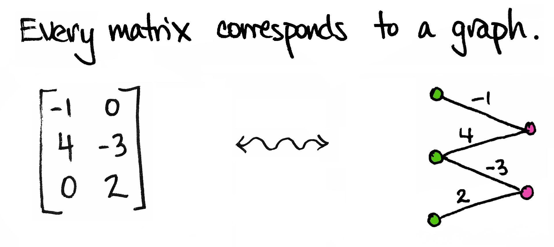
To start, I'll be a little more precise: every matrix corresponds to a weighted bipartite graph. By "graph" I mean a collection of vertices (dots) and edges; by "bipartite" I mean that the dots come in two different types/colors; by "weighted" I mean each edge is labeled with a number.
The graph above corresponds to a $3\times 2$ matrix $M$. You'll notice I've drawn three ${\color{Green}\text{green}}$ dots—one for each row of $M$—and two ${\color{RubineRed}\text{pink}}$ dots—one for each column of $M$. I've also drawn an edge between a green dot and a pink dot if the corresponding entry in $M$ is non-zero.

For example, there's an edge between the second green dot and the first pink dot because $M_{21}=4$, the entry in the second row, first column of $M$, is not zero. Moreover, I've labeled that edge by that non-zero number. On the other hand, there is no edge between the first green dot and the second pink dot because $M_{12}$, the entry in the first row, second column of the matrix, is zero.
Allow me to describe the general set-up a little more explicitly.
Any matrix $M$ is an array of $n\times m$ numbers. That's old news, of course. But such an array can also be viewed as a function $M\colon X\times Y\to\mathbb{R}$ where ${\color{Green}X}=\{x_1,\ldots,x_n\}$ is a set of $n$ elements and ${\color{RubineRed}Y}=\{y_1,\ldots,y_m\}$ is a set of $m$ elements. Indeed, if I want to describe the matrix $M$ to you, then I need to tell you what each of its $ij$th entries are. In other words, for each pair of indices $(i,j)$, I need to give you a real number $M_{ij}$. But that's precisely what a function does! A function $M\colon X\times Y\to\mathbb{R}$ associates for every pair $(x_i,y_j)$ (if you like, just drop the letters and think of this as $(i,j)$) a real number $M(x_i,y_j)$. So simply write $M_{ij}$ for $M(x_i,y_j)$.
Et voila. A matrix is a function.

As suggested, let's further think of $X$'s elements as being ${\color{Green}\text{green}}$ and $Y$'s elements as being ${\color{RubineRed}\text{pink}}$. Then a matrix $M$ corresponds to a weighted bipartite graph in the following way: the vertices of the graph have two different colors provided by ${\color{Green}X}$ and ${\color{RubineRed} Y}$, and there is an edge between every $x_i$ and $y_j$ which is labeled by the number $M_{ij}$. But if this number is zero, then simply omit that edge.
Et voila. Every matrix corresponds to a graph.
Nice things happen when we visualize matrices in this way. For instance...
Matrix multiplication corresponds to traveling along paths.
Given two matrices (graphs) $M\colon {\color{Green}X}\times {\color{RubineRed}Y}\to\mathbb{R}$ and $N\colon {\color{RubineRed}Y}\times {\color{ProcessBlue}Z}\to\mathbb{R}$, we can multiply them by sticking their graphs together and traveling along paths: the $ij$th entry of $MN$, i.e. the value of the edge connecting $x_i$ to $z_j$, is obtained by multiplying the edges along each path from $x_i$ to $z_j$ and adding them together. For example:

Symmetric matrices correspond to symmetric graphs.
A matrix is symmetric if it is equal to its transpose. That symmetry is always seen by reflecting across the diagonal of the matrix. But you can also see the symmetry in the graph. In particular, the graph makes it visually intuitive why $MM^\top$ and $M^\top M$ are always symmetric, for any $M$!

Matrices with all nonzero entries correspond to complete bipartite graphs.
If none of the entries of a matrix is zero, then there are no missing edges in its corresponding graph. That means every vertex in $X$ is connected to every vertex in $Y$. Such bipartite graphs are called complete.

Block matrices correspond to disconnected graphs.
More specifically, the block matrix obtained from a direct sum corresponds to a disconnected graph. The direct sum of two matrices is obtained by stacking them together into one larger array. (Not unlike the direct sum of vectors.) The result is a big block matrix with zero-blocks. The graph of that matrix is obtained by stacking the graphs of the original matrices together.

We could say more about matrices and graphs, but I'd like to steer the conversation in a slightly different direction. As it turns out, probability fits in very nicely with our matrix-graph discussion. It does so by way of another nice little fact:

For example:

The graphs of such probability distributions allow us to read off some nice things.
Joint Probability
By construction, the edges of the graph capture the joint probabilities: the probability of $(x_i,y_j)$ is the label on the edge connecting them.

Marginal Probability
Marginal probabilities are obtained by summing along the rows/columns of the matrix (equivalently, of the chart above). For example, the probability of $x_1$ is $p(x_1)=p(x_1,y_1)+p(x_1,y_2)=\frac{1}{8}+0$, which is the sum of the first row. Likewise, the probability of $y_2$ is $p(y_2)=p(x_1,y_2)+p(x_2,y_2)+p(x_3,y_2)=0+\frac{1}{8}+\frac{1}{4}$, which is the sum of the second column.
In the graph, the marginal probability of $x_i$ is the sum of all edges that have $x_i$ as a vertex. Similarly, the marginal probability of $y_j$ is the sum of all edges that have $y_j$ as a vertex.

Conditional Probability
Conditional probabilities are obtained by dividing a joint probability by a marginal probability. For example, the probability of $x_3$ given $y_2$ is $p(x_3\vert y_2)=\frac{p(x_3,y_2)}{p(y_2)}$. In the graph, this is seen by dividing the edge joining $x_3$ and $y_2$ by the sum of all edges incident to $y_2$. Likewise, the conditional probability of some $y_i$ given $x_j$ is the value of the edge joining the two, divided by the sum of all edges incident to $x_j$.

Pretty simple, right?
There's nothing sophisticated here, but sometimes it's nice to see old ideas in new ways!

Relations as Matrices
I'll close this post with an addendum—another simple fact that I think is really delightful, namely: matrix arithmetic makes sense over commutative rings. Not just fields like $\mathbb{R}$ or $\mathbb{C}$. In fact, it gets better. You don't even need negatives to multiply matrices: matrix arithmetic makes sense over commutative semi-rings! (A semi-ring is a ring without additive inverses.)
I think this is so delightful because the set with two elements $\mathbb{Z}_2=\{0,1\}$ forms a semi-ring with the following addition and multiplication operations:

Why is this so great? Because a matrix $M\colon X\times Y\to\mathbb{Z}_2$ is the same thing as a relation. A relation is just the name for a subset $R$ of a Cartesian product $X\times Y$. In other words, every $\mathbb{Z}_2$-valued matrix defines a relation, and every relation defines a $\mathbb{Z}_2$-valued matrix: $M_{ij}= 1$ if and only if the pair $(x_i,y_j)$ is an element of the subset $R$, and $M_{ij}= 0$ otherwise.

The graphs of matrices valued in $\mathbb{Z}_2$ are exactly like the graphs discussed above, except now the weight of any edge is either 0 or 1. If the weight is 0 then, as before, we simply won't draw that edge.
(By the way, you can now ask, "Since every relation corresponds to a matrix in $\mathbb{Z}_2$, what do matrices corresponding to equivalence relations look like?" But I digress....)
By changing the underlying (semi)ring from $\mathbb{R}$ to $\mathbb{Z}_2$, we've changed the way we interpret the weights. For instance, in the probabilistic scenario above, we could've asked, "What's the probability of getting from $x_1$ to $y_1$?" The answer is provided by the weight on the corresponding edge, in that case: 12.5%. Alternatively, when the matrix is valued in $\mathbb{Z}_2$, the question changes to: "Is it possible to get from $x_1$ to $y_1$?" The answer is Yes if the edge is labeled by 1, and it's No if the edge is labeled by 0. (This nice idea has been explained in various places, like here for instance.)
What's great is that composition of relations is exactly matrix multiplication using the $\mathbb{Z}_2$ arithmetic above. In other words, given any two relations $R\subset X\times Y$ and $S\subset Y\times Z$, there is a new relation $SR\subset X\times Z$ consisting of all pairs $(x,z)$ such that there exists at least one $y\in Y$ with $(x,y)\in R$ and $(y,z)\in S$. This new relation is exactly that specified by the product of the matrices representing $R$ and $S$.

This little fact about matrices/relations is definitely at the top of my list of favorite-math-facts.* One reason is because the category of finite sets and relations is a lot like the category of finite vector spaces and linear maps. Actually, it's more like the category of finite-dimensional Hilbert spaces. And that means that a lot of seemingly disparate ideas all of the sudden become closely related. The connections can be made more precise, and it's a story that's often shared in the category theory community. Hopefully I'll get around to sharing it here on the blog, too.
*Relations are often under-appreciated, I think. In high school, I learned that functions are of utmost importance. "Assignments must only have one output for each input," they said. No one ever mentioned anything about multiple outputs. Whenever such an anomaly did crop up, it was usually presented as abnormal and off-limits. But relations deserve much better treatment! One reason is because relations are to sets what linear maps are to vector spaces. There's a lot of juice in linear algebra, so there's a lot of juice in relations too. In short, relations are very much top-notch citizens.
New! [Added October 20, 2019] You can see some of today's ideas in action in "Modeling Sequences with Quantum States" (arXiv:1910.07425). There, we represent matrices as bipartite graphs to keep track of some of the combinatorics involved in a certain training algorithm. You can read more about this work with Miles Stoudenmire and John Terilla here on the blog.