Welcome back to our mini-series on quantum probability! Last time, we motivated the series by pondering over a thought from classical probability theory, namely that marginal probability doesn't have memory. That is, the process of summing over of a variable in a joint probability distribution causes information about that variable to be lost. But as we saw then, there is a quantum version of marginal probability that behaves much like "marginal probability with memory." It remembers what's destroyed when computing marginals in the usual way. In today's post, I'll unveil the details. Along the way, we'll take an introductory look at the mathematics of quantum probability theory.

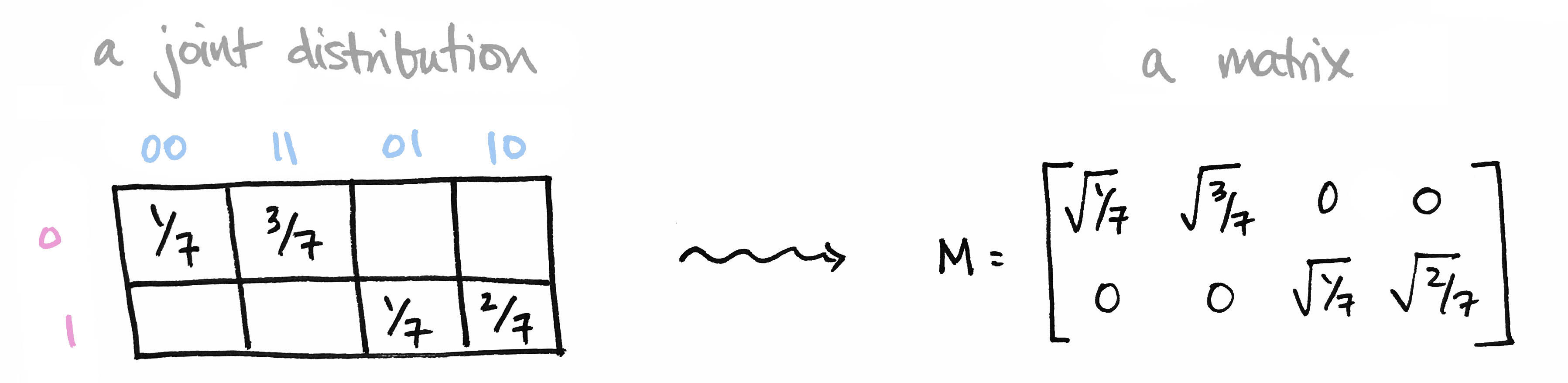
Let's begin with a brief recap of the ideas covered in Part 1: We began with a joint probability distribution on a product of finite sets $p\colon X\times Y\to [0,1]$ and realized it as a matrix $M$ by setting $M_{ij} = \sqrt{p(x_i),p(y_j)}$. We called elements of our set $X=\{0,1\}$ prefixes and the elements of our set $Y=\{00,11,01,10\}$ suffixes so that $X\times Y$ is the set of all bitstrings of length 3.

We then observed that the matrix $M^\top M$ contains the marginal probability distribution of $Y$ along its diagonal. Moreover its eigenvectors define conditional probability distributions on $Y$. Likewise, $MM^\top$ contains marginals on $X$ along its diagonal, and its eigenvectors define conditional probability distributions on $X$.

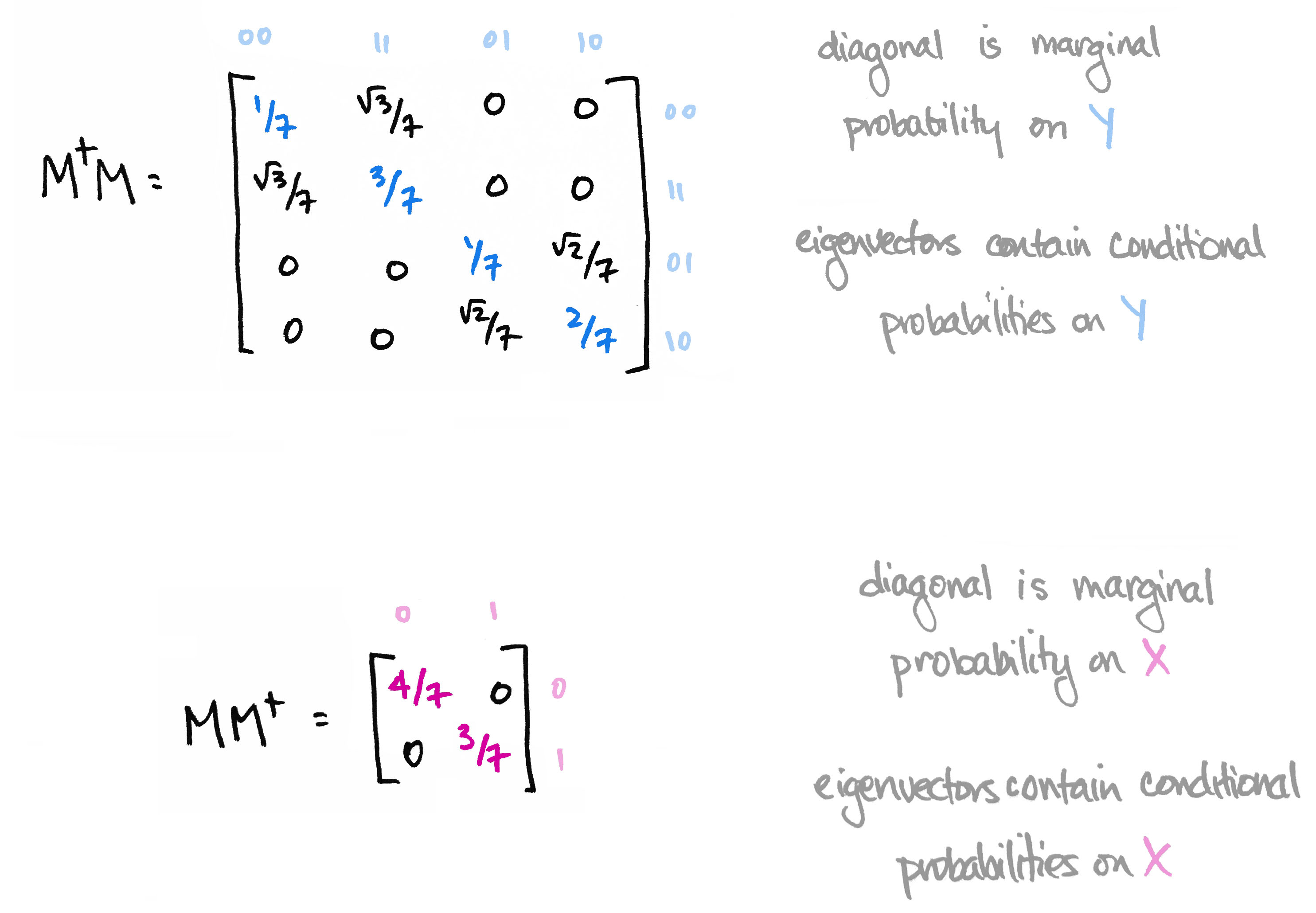
The information in the eigenvectors of $M^\top M$ and $MM^\top$ is precisely the information that's  destroyed when computing marginal probability in the usual way. The big reveal last time was that the matrices $M^\top M$ and $MM^\top$ are the quantum versions of marginal probability distributions.

As we'll see today, the quantum version of a probability distribution is something called a density operator. The quantum version of marginalizing corresponds to "reducing" that operator to a subsystem. This reduction is a construction in linear algebra called the partial trace. I'll start off by explaining the partial trace. Then I'll introduce the basics of quantum probability theory. At the end, we'll tie it all back to our bitstring example.

In this article and the next, I'd like to share some ideas from the world of quantum probability.* The word "quantum" is pretty loaded, but don't let that scare you. We'll take a first—not second or third—look at the subject, and the only prerequisites will be linear algebra and basic probability. In fact, I like to think of quantum probability as another name for "linear algebra + probability," so this mini-series will explore the mathematics, rather than the physics, of the subject.**

In today's post, we'll motivate the discussion by saying a few words about (classical) probability. In particular, let's spend a few moments thinking about the following: ‍

What do I mean? We'll start with some basic definitions. Then I'll share an example that illustrates this idea.

A probability distribution (or simply, distribution) on a finite set $X$ is a function $p \colon X\to [0,1]$ satisfying $\sum_x p(x) = 1$. I'll use the term joint probability distribution to refer to a distribution on a Cartesian product of finite sets, i.e. a function $p\colon X\times Y\to [0,1]$ satisfying $\sum_{(x,y)}p(x,y)=1$. Every joint distribution defines a marginal probability distribution on one of the sets by summing probabilities over the other set. For instance, the marginal distribution $p_X\colon X\to [0,1]$ on $X$ is defined by $p_X(x)=\sum_yp(x,y)$, in which the variable $y$ is summed, or "integrated," out. It's this very process of summing or integrating out that causes information to be lost. In other words, marginalizing loses information. It doesn't remember what was summed away!

I'll illustrate this with a simple example. To do so, I need to give you some finite sets $X$ and $Y$ and a probability distribution on them.

In the previous post, I described a simple way to think about matrices, namely as bipartite graphs. Today I'd like to share a different way to picture matrices—one which is used not only in mathematics, but also in physics and machine learning. Here's the basic idea. An $m\times n$ matrix $M$ with real entries represents a linear map from $\mathbb{R}^n\to\mathbb{R}^m$. Such a mapping can be pictured as a node with two edges. One edge represents the input space, the other edge represents the output space.

That's it!

We can accomplish much with this simple idea. But first, a few words about the picture: To specify an $m\times n$ matrix $M$, one must specify all $mn$ entries $M_{ij}$. The index $i$ ranges from 1 to $m$—the dimension of the output space—and the index $j$ ranges from 1 to $n$—the dimension of the input space. Said differently, $i$ indexes the number of rows of $M$ and $j$ indexes the number of its columns. These indices can be included in the picture, if we like:

This idea generalizes very easily. A matrix is a two-dimensional array of numbers, while an $n$-dimensional array of numbers is called a tensor of order $n$ or an $n$-tensor. Like a matrix, an $n$-tensor can be  represented by a node with one edge for each dimension.

A number, for example, can be thought of as a zero-dimensional array, i.e. a point. It is thus a 0-tensor, which can be drawn as a node with zero edges. Likewise, a vector can be thought of as a one-dimensional array of numbers and hence a 1-tensor. It's represented by a node with one edge. A matrix is a two-dimensional array and hence 2-tensor. It's represented by a node with two edges. A 3-tensor is a three-dimensional array and hence a node with three edges, and so on.

Today I'd like to share an idea. It's a very simple idea. It's not fancy and it's certainly not new. In fact, I'm sure many of you have thought about it already. But if you haven't—and even if you have!—I hope you'll take a few minutes to enjoy it with me. Here's the idea:

So simple! But we can get a lot of mileage out of it.

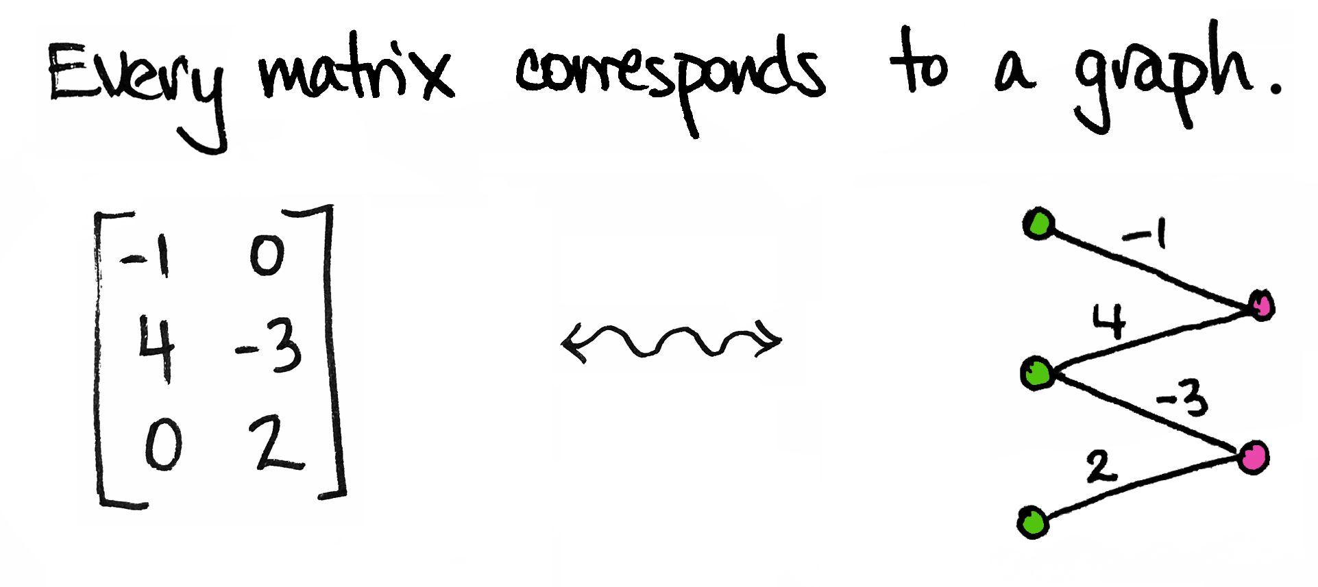
To start, I'll be a little more precise: every matrix corresponds to a weighted bipartite graph. By "graph" I mean a collection of vertices (dots) and edges; by "bipartite" I mean that the dots come in two different types/colors; by "weighted" I mean each edge is labeled with a number.

The graph above corresponds to a $3\times 2$ matrix $M$. You'll notice I've drawn three ${\color{Green}\text{green}}$ dots—one for each row of $M$—and two ${\color{RubineRed}\text{pink}}$ dots—one for each column of $M$. I've also drawn an edge between a green dot and a pink dot if the corresponding entry in $M$ is non-zero. 

For example, there's an edge between the second green dot and the first pink dot because $M_{21}=4$, the entry in the second row, first column of $M$, is not zero. Moreover, I've labeled that edge by that non-zero number. On the other hand, there is no edge between the first green dot and the second pink dot because $M_{12}$, the entry in the first row, second column of the matrix, is zero.

Allow me to describe the general set-up a little more explicitly.

Once upon a time, we embarked on a mini-series about limits and colimits in category theory. Part 1 was a non-technical introduction that highlighted two ways mathematicians often make new mathematical objects from existing ones: by taking a subcollection of things, or by gluing things together. The first route leads to a construction called a limit, the second to a construction called a colimit.

The formal definitions of limits and colimits were given in Part 2. There we noted that one speaks of "the (co)limit of [something]." As we've seen previously, that "something" is a diagram—a functor from an indexing category to your category of interest. Moreover, the shape of that indexing category determines the name of the (co)limit: product, coproduct, pullback, pushout, etc.

In today's post, I'd like to solidify these ideas by sharing some examples of limits. Next time we'll look at examples of colimits. What's nice is that all of these examples are likely familiar to you—you've seen (co)limits many times before, perhaps without knowing it! The newness is in viewing them through a categorical lens. 

‍